In the previous two issues, we assessed The Sky Imaging Edition’s (TSIE’s) capabilities for creating an equatorial-mount pointing model using ‘TPoint’, and tested its functionality during autofocusing and autoguiding. TSIE comes with TPoint included, in addition to a ‘Camera Add-on’ that allows full control of CCD cameras along with autoguiders, focusers, filter-wheels, rotators and dome control. So in this final part of my exploration of TSIE’s capabilities, I’ll assess how it performs during an imaging run, and cover some of the software’s new features.
Easy connections
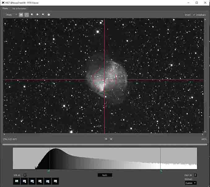
After firing up TSIE on my observatory laptop, it took only a minute or so to connect all of my imaging devices to it and to cool my QSI 683wsg CCD camera to an operating temperature of –15 degrees Celsius. I chose a nice, easy first target, M27, the famous Dumbbell Nebula in the constellation of Vulpecula. Figure 1 shows the zoomed-in field after slewing onto the target. The central star was offset by a tiny amount and I didn’t feel the need for any further accuracy. I’d called upon the @Focus2 autofocusing routine to focus the image and it did a great job first time (see last issue for details on both @Focus2 and @Focus3).
After downloading a dark-subtracted image, which was taken with my Starlight Xpress Lodestar guide camera, I was able to choose a suitable star for guiding. The sensitivity of the Lodestar coupled with the QSI camera’s integral off-axis guider port means that it’s always possible to find a guide star with exposures of around five seconds. I shot a few two-minute exposures with a luminance filter to ensure that all was well and by that point M27 was nearing the meridian. After a full meridian flip, M27 appeared with just a tiny offset from the crosshair centre, so I shot a 10-minute exposure to use as a luminance file and I combined it with the earlier two-minute exposures.
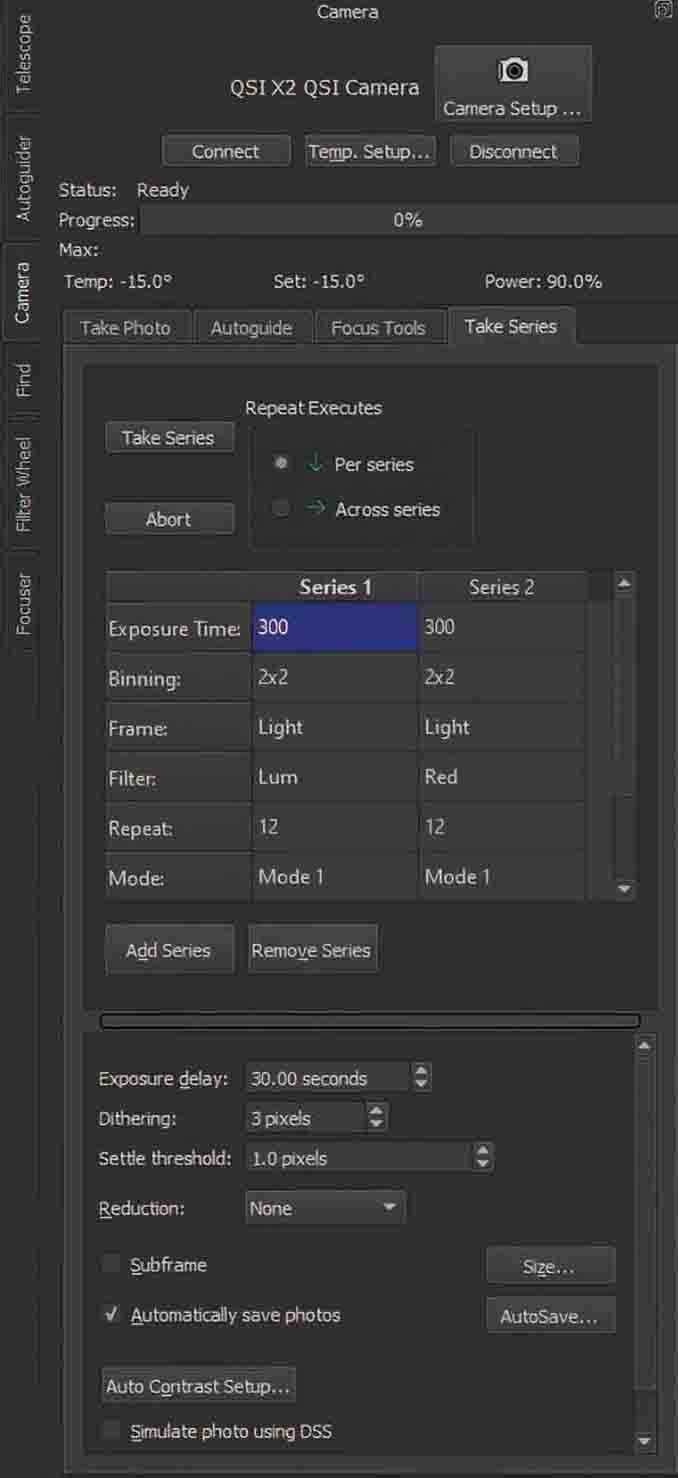
Next, I planned to take a sequence of images through red, green and blue filters. When imaging the deep sky, most astrophotographers take long sequences of exposures that will be calibrated, aligned and stacked to produce a master light-frame. The exposure sequence can be automated and in TSIE it’s done using the ‘Take Series’ tab in the ‘Camera’ menu. Figure 2 shows the menu with the Take Series tab selected. At centre is where the sequence is set up. Clicking on any of the fields, such as the ‘exposure duration’ shown in blue, allows a particular preference to be inserted, in this case 300 seconds for the exposure time. Below that are binning, type of frame (i.e. dark, light, flat, etc.), filter, how many frames to take (repeat), and a choice of calibration frame to be used. I left this on none, to apply my own calibrations later. Clicking on ‘Add Series’ does just that and, for Series 2, I left everything the same but changed the filter setting to red. I then created two additional series, set up for the green and blue filters. There’s a choice to use ‘Per series’, which in our case would capture and save twelve 300-second exposures through the luminance filter, or ‘Across series’, which would take a 300-second exposure through the luminance filter and then change to the red, green and blue filters consecutively. I left this on Per Series.
Below that are options to set up dithering. This is an important procedure to use. Basically, the mount is offset by a few pixels at the end of every exposure so that when the images are aligned, noise in the images is also offset rather than stacking up in registration. During the stacking process (using stars for alignment), a reference frame is chosen and usually this is the frame with the best tracking and FWHM values. After comparison with the reference frame, noise in the remaining images is more easily subtracted and replaced with average-value pixels, producing a much cleaner image.
As seen in Figure 2, when setting up the dithering procedure I used a shift of three pixels. It’s also critical to use an exposure delay to allow the guiding to settle after dithering has occurred, and for this I chose thirty seconds.
File names
The ‘Automatically save photos’ box must be ticked, and then clicking on the ‘AutoSave’ button opens a menu where you can choose a file location for the images to be saved to. I found this menu to be a bit awkward because without user-intervention the file name for each image was long and clunky. Fortunately, under the ‘Customize AutoSave File Names’, you can include useful descriptions in each saved-file name. The ‘Abbreviations Key’ information at the bottom lists available options that can be used (see Figure 3). I first chose the subject title from the ‘File name prefix’, in this case M27. Then under the ‘Light frames’ field I typed :b :e :f :l and this inserted, respectively, binning status, exposure time in seconds, filter name, and image type (a light frame in this case). A resulting file name in this sequence would be, for example, M27 2×2 Blue 300 L 00000001.fit.
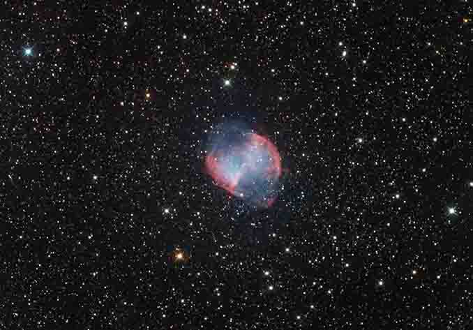
Within the menu, under the ‘Sample AutoSave file name’ field, you can see a preview of the file name with the chosen parameters before starting the series capture. Each series records the appropriate filter used, making it easy to differentiate the images when applying calibrations and stacking at a later date. Clicking on the ‘Take Series’ button at top left initiates the imaging sequence. Although I used a very small imaging run (hence the choice of a bright target), the sequence worked flawlessly, producing the LRGB image of M27 shown in Figure 4.

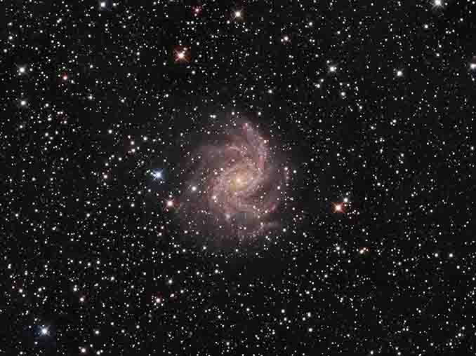
As the sky conditions were so good, I slewed onto NGC 6946, which is a lovely face-on spiral galaxy in Cygnus. Since it is a fairly bright galaxy, I initiated another short imaging run using LRGB filters. The resulting image after processing is shown in Figure 5. After a couple of nights using TSIE, I found that the interface became quite intuitive to use and navigate. There was a lot of switching between tabs to access different devices, but it all became quite natural to use and it was great to have all aspects of the imaging and telescope control within the same program. Also highly commendable was the fact that at all times TSIE was completely stable, with no crashes or hanging, or any form of delay when switching between devices.
Collimation
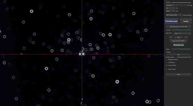
TSIE has some new features that are worth mentioning. The first is a collimation tool to assess the alignment of mirrors in a reflecting telescope. The tool is located in the Camera menu under ‘Focusing Tools’ (the same location as @Focus2 and @Focus3). Clicking on the ‘Collimation’ button launches the view shown in Figure 6. At the centre is a defocused image of the star Alpheratz (alpha [α] Andromedae). At top right of the screen is where the exposure, binning and filter are chosen. Clicking on the ‘Take Sample’ button takes an image and displays it on the screen. Clicking on the ‘Loop’ button runs a continuous series of images. I used my Paramount’s hand paddle to gently nudge the star images to the centre of the screen and then adjusted the size of the red rings to match as closely as possible the inner and outer edges of the defocused star. This helps with assessing the circularity of the star image and whether the secondary mirror is positioned at the centre. The ring dimensions are adjusted using the two sliders at the bottom of the screen. When a star is selected, you can zoom in and create a sub-frame that matches the zoomed view, speeding up download times. It’s also possible to save the focuser’s current position, defocus the star for assessment and then return the focuser to its starting position. The menu also incorporates autofocusing using the brilliant @Focus3 routine. This is definitely a handy tool to do a quick check on the collimation of your mirrors.

Into the corners
There are three buttons at lower right: ‘Inspection Mode’, which shows the star without the crosshairs; ‘Crosshairs’, which gives the view shown in Figure 6; and ‘Four corners’, which splits the view to show the corners of the sensor to allow you to check for image planarity. I slewed my telescope onto the Double Cluster in Perseus and took a seven-second exposure with a luminance filter. That placed plenty of stars in the field of view (Figure 7). The user manual suggests defocusing star images and then adjusting the image plane if possible (some cameras have tip-tilt adjusters for this purpose) until all the out-of-focus stars appear the same size in each corner. The stars in this image looked pretty similar in size but I noticed a few non-circular outliers. I suspect these were caused by my focal reducer but they could also be the result of the quality of the main telescope’s optics tailing off in the extreme corners.
Live stacking for public events
Another nice new feature is the live-stacking tool, which is accessed under the Camera menu. Clicking on the ‘Take Photo’ tab opens another menu and then clicking on ‘Live Stack’ brings up the screen shown in Figure 8. The purpose of this tool is to take multiple exposures that are aligned and stacked on-the-fly to build up a strong image. To test this I slewed the telescope onto M31, the magnificent Andromeda Galaxy, and from the options given at the top right of the screen I selected an exposure time of 30 seconds with the camera binned 2 × 2 through a luminance filter. I’d taken suitable dark and flat-field images before starting the live stack, so I loaded them using the ‘Calibration Frames’ button at top right. Clicking on the big ‘Start!’ button initiated the procedure. As the first frame downloaded, it appeared on the screen looking quite good. As the second image downloaded, it was automatically aligned and stacked, and so on. At upper right is an ‘Images’ readout, where the number of images taken is displayed and also how much the noise component has been reduced.
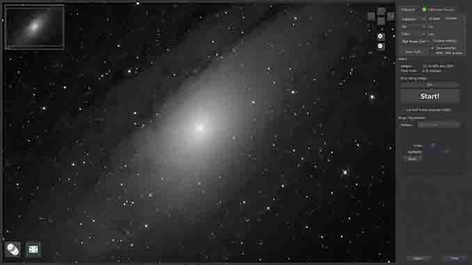
The whole purpose of stacking images is to reduce noise. The signal component of stars, galaxies, etc., adds in a linear sense, whereas the noise component only adds as the square root of the total number of images taken, so taking lots of images results in a great signal-to-noise ratio. I shot thirteen images and was informed that there was 72.26 per cent less noise compared to a single 30-second exposure. When the sequence finished, I saved the image as a FITS file. You can also elect to save each of the individual FITS images. I think this tool would be great for observatory open evenings, where many people can see the image building up on screen. It’s possible to take images with a one-shot colour camera and see a colour image continuing to improve as more and more sub-frames are taken. Objects like the Orion Nebula would work well in this context.
I experienced three hugely enjoyable nights putting The Sky Imaging Edition through its paces. As an integrated package, it worked flawlessly, and it was easy to switch between controlling the imaging equipment and controlling the telescope. As mentioned earlier, the product is stable and efficient. Is it worth its steep $595 price tag? For sure it’s a considerable outlay, especially given that it is in competition with free programs such as N.I.N.A. and APT (Astro Photography Tool),but considering the power of TPoint for mount modelling and polar-alignment assistance, complete hardware functionality and a brilliant planetarium package, I think it is definitely good value for the money.
At a glance
Minimum system requirements
macOS: 2GHz Intel Core Duo or faster, macOS Sierra (10.12), High Sierra (10.13), Mojave (10.14) or Catalina (10.15) 512MB RAM, 64MB video RAM, 2.5GB disk space
Windows: 1.5GHz or faster, Intel Pentium 4, Pentium M, Pentium D or better, or AMD K-8 (Athlon) or better, Windows 10, 512MB RAM, 128MB video RAM, 2.5GB disk space
Linux: A computer running 64-bit x86 Linux Ubuntu 12.04 LTS or later, Ubuntu GUI and OpenGL, 512MB RAM, 2GB minimum disc space
Raspberry Pi: Third-generation Raspberry Pi device (Raspberry Pi 3 Model B or later) SanDisk Ultra PLUS 16GB microSDHC UHS-1 card, 2GB minimum free space, Well-ventilated project case (fan not necessary) Optional external 9-pin serial port
Price: $595
Details: bisque.com