Last issue we assessed The Sky Imaging Edition’s (TSIE’s) capabilities in creating a precise pointing model for equatorial mounts using its TPoint module. This new edition of The Sky comes with both TPoint and the Camera Add-on. The latter allows for the integration of imaging cameras, autoguiders, filter-wheels, focusers and so on to the planetarium software used for controlling equatorial mounts and navigating around the sky. With a model containing just 61 stars, I was able to significantly improve the accuracy of my Paramount ME equatorial mount.
Auto-focusing in TSIE
This issue, I’d like to assess how well TSIE performs when autoguiding, as well as judging its autofocusing accuracy. We’ll start with the latter. Attaining sharp focus is incredibly difficult and is a make-or-break decider of image quality. It’s also essential for any scientific imaging such as photometry. The point of best focus in an imaging system is known as ‘critical focus’. This is a zone of sharp focus that is smaller in ‘fast’ optical systems with steep light cones, making fast telescopes more difficult to focus. The critical focus zone is calculated by multiplying the square of the focal ratio by 2.2, with the result delivered in microns.
Using my GSO 254mm Ritchey–Chrétien telescope, equipped with a 0.67× focal reducer, I have an f-ratio of f/5.3 (and a focal length of 1,340mm). Inserting this into the calculation gives 5.32 × 2.2 = 61.8 microns.
This is a preposterously small focus zone. For those that prefer ‘real world’ figures, it equates to 0.0618mm. As the f-ratio increases, the critical focus zone becomes wider. With my telescope imaging without the focal reducer at f/8, the critical focus zone enlarges to 0.14mm. Unsurprisingly, the use of a good quality electronic focuser is required to obtain the best results.
TSIE features some good tools for attaining sharp focus. The first, known as ‘@Focus2’, is a comprehensive automatic focusing routine that slews to a star of appropriate brightness, places a small sub-frame around the star, computes a suitable exposure time and then finds the critical focus. I don’t think @Focus2 has changed much since my review of an earlier edition of The Sky in 2018, so I was able to use the same parameters as before and they worked extremely well.
To set up the focusing run, you need to click on ‘Focus Tools’ in the Camera menu. From here there is a choice of using two focusing aids, @Focus2 or a new addition, @Focus3 (more of which shortly).
Focus range
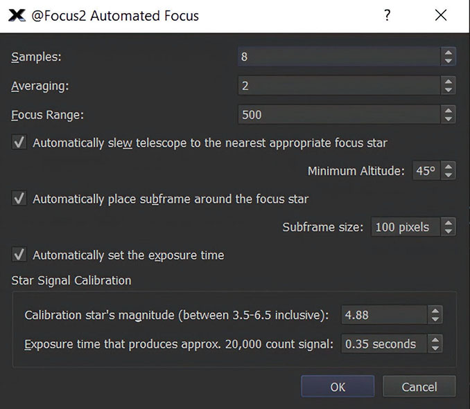
Figure 1 lists the parameters that I selected for use with my Moonlite focuser. ‘Samples’ is the total number of images taken for both sides of the optimal focus position and for this I chose eight (i.e. four each side). ‘Averaging’ is the number of images taken per focus sample, so for each of the eight samples I chose, the software can take multiple images before moving the focuser. The reason for this is that if the seeing is poor, multiple images can be averaged to produce a truer value. I selected two for this. ‘Focus Range’ is a little more complex and requires some user input to get the best results with any particular focuser. The user manual (which is very well written and comprehensive, but slightly out of date) states that best results come from using a value that is approximately 40× the size of the critical focus zone. For my set up, this is 40 × 61.8 = 2,472. This number then has to be divided by the distance-per-step figure of a particular focuser. Unfortunately, I was unable to remember the step-size of my focuser, so I went online and found a similar model that had a step-size of 4.06 microns. Dividing 2,468 by 4.06 gives a value of 608. I’d initially guessed a value of 500 for the Focus Range and it worked well.
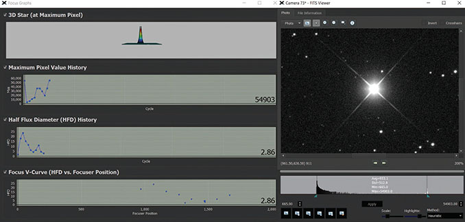
Figure 2 shows the results of the first focusing run. The graphs look a bit ragged but the ‘Maximum Pixel Value History’ and ‘Half Flux Diameter (HFD) History’ are moving in the right direction. The ‘Focus V-Curve’ certainly isn’t a smooth ‘V’ shape, but the point of best focus was pretty accurate. I immediately shot a 30-second exposure of the focus star and using the ‘Heuristic display mode’ I was able to check that the star images were crisp and the long diffraction spikes were single. I ran the autofocus routine several times and in most cases it returned a very similar result, although it also failed a few times. If nothing else, this underlines that autofocusing is a complicated procedure.
Next, I clicked on @Focus3. I couldn’t find any information about this new feature in the user manual, but I located a PDF on the Software Bisque website that explained how the routine works. Intriguingly, it doesn’t rely on a star’s half-flux diameter or FWHM measurement, but instead makes a contrast/sharpness-based assessment, which I presume is how modern auto-focus camera lenses work. Even better, it purports to be able to focus on a field of stars, galaxies, nebulae and Solar System objects (with filters). The advantage of this is that you can remain on your imaging target, refocus and then continue. Astonishingly, you can also focus on daytime targets.
Search span
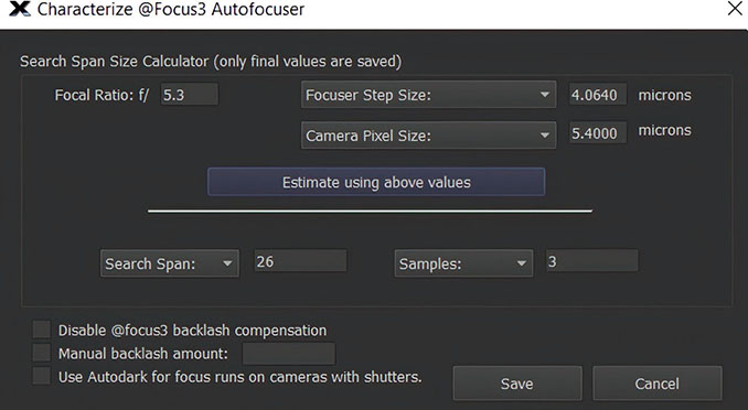
The system is pretty well automated, but once again requires some user input. Figure 3 shows the options. I typed 5.3 in the ‘Focal Ratio’ field. For ‘Focuser Step Size’, I clicked on the downward arrow and it opened a list of focusers including two Moonlite options. Happily, one of them inserted a step-size of 4.0640 microns, which was the value I’d used on the previous test. For ‘Camera Pixel Size’ I was able to choose my imaging sensor from the small list that opened, using a value of 5.4 microns. With these parameters, the software computed a ‘Search Span’ of 26, meaning that each move of the focuser was in increments of 26 steps. The ‘Samples’ option allows additional images to be taken at a specific focuser position (similar to @Focus2) which, when averaged, give more accurate data points in poor seeing.
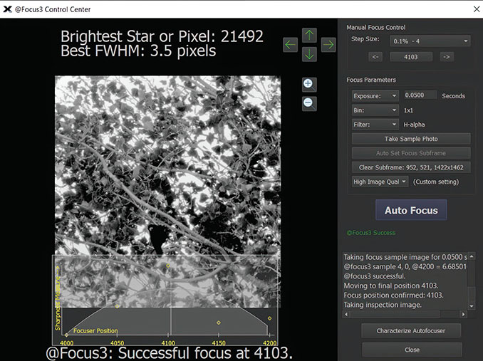
As the camera moves in and out of focus, the sharpness of the star image is plotted as a bell-shaped or ‘Gaussian’ curve. The top point of the curve is the region of sharpest focus. Provided that there are a minimum of five data points within the curve, then the routine will work. I just had to try this routine on a daytime target, so in the afternoon I slewed the telescope onto a distant tree and, using a hydrogen-alpha filter and a very short exposure, I was able to get a useable image. Figure 4 shows this within the @Focus3 Control Centre. In this menu you can choose a suitable exposure time (@Focus3 will modify this if necessary), binning and filter.
Clicking on ‘Take Sample Photo’ takes an image using your settings. At the top of the menu is a readout of the brightest star or pixel in the image, so that you can be sure the focus star isn’t saturated. The ‘+’ or ‘–‘ zoom buttons at upper centre allow zooming in or out and, if you’ve zoomed in, clicking on ‘Set Subframe to Current View’ takes a new image that is sized at the zoom level, speeding up download times.
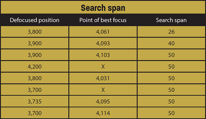
At the bottom of the menu is a graphical representation of the procedure, with the data points placed along what we can call an ‘A-Curve’. Next, I ran the focusing sequence several times with the camera manually defocused beforehand to test whether the point of best focus was reproducible. The accompanying table (above) lists the results. I also adjusted the ‘Search Span’ figure and this is shown in the table’s right-hand column.
The two X’s mark where the focus routine failed. The first was because of my focuser reaching the end of travel. I’d had to move the focuser by several thousand steps to get the tree in focus, so this wasn’t surprising. I’m not sure why the second failure occurred. However, the point of best focus was pretty consistent bearing in mind the warm afternoon sunshine and probable air currents. I found it to be very impressive. I continued the test by slewing onto a bright star (in broad daylight) and running the routine from either side of focus and it worked every time.
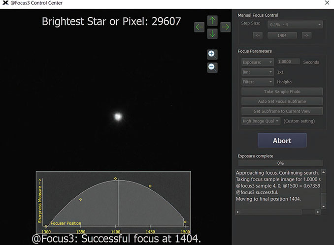
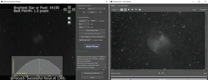
Later that evening I was able to test @Focus3 on the night sky. Figure 5 shows the result obtained by using a bright star and a one-second exposure with a hydrogen-alpha filter. To confirm the focus, I took longer test exposures after every run and they seemed pretty sharp. My next test involved taking a short exposure of M27, the Dumbbell Nebula, and running the auto-focus routine on the whole frame rather than just a zoomed-in section. I used an exposure time of just five seconds and binned the camera 2 × 2 with a luminance filter. After a few moments @Focus3 announced that it had made a successful focus (Figure 6 left-hand side, overleaf) and I took a 30-second exposure (with a single dark frame but no flat field), which is shown on the right of Figure 6 and looks absolutely fine.
I have to admit to being hugely impressed by both of these focusing routines. Once I became familiar with the user-parameters and methodology, I found that they both worked extremely well – top marks!
Calibration and autoguiding
Autoguiding is an important part of long-exposure deep-sky imaging. For success, a calibration procedure must be carried out to match the guide camera with the tracking mount. This usually involves centring a suitable star on the guider and instructing the mount to move in +x, –x, +y and –y directions. By doing this procedure, the mount will know how far to move when making a guiding correction. TSIE supports autoguiding using a relay cable between the guide camera and mount or via ‘pulse’ guiding without a cable. Both instances require calibration to be completed first. The ‘Autoguide Setup’ menu is where you set a suitable calibration time. By this I mean the time that it takes to move the guide star a suitable distance and not off the edge of the sensor. This menu is where the type of guiding is chosen (via a relay cable or pulse) and the ‘aggressiveness’ of the tracking corrections (the default amount, 10 being 100 per cent correction, but this can be lowered if the tracking is over-correcting).
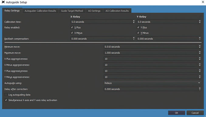
Figure 7 shows the Autoguide Setup menu. I carried out the first guider calibration using a relay cable and selected calibration move times of five seconds. The left-hand pane of Figure 8 shows a successful guider calibration. The green calibration vectors were slightly offset from the x and y axes, showing that my Starlight Xpress Lodestar guide camera was not positioned orthogonally on the guide camera port of my QSI 683wsg CCD camera. This wasn’t a problem as TSIE can guide happily in any orientation. One thing to bear in mind, though, if you are using an uncooled guide camera that generates ‘hot’ pixels (defective pixels that are saturated and so are very bright) is that these rogues can be mistaken for the guide star during both calibration and autoguiding. The way round this is to ensure that a dark frame is taken that records and subtracts the hot pixels. I did this but found that the fiends were still visible, so I had to choose a much brighter guide star. I also created a master dark frame from eight sub-exposures with the Lodestar guide camera and set it to automatically calibrate every subsequent light frame used for guiding, which helped.
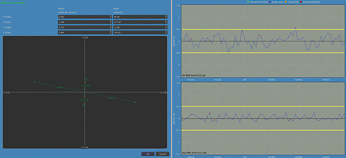
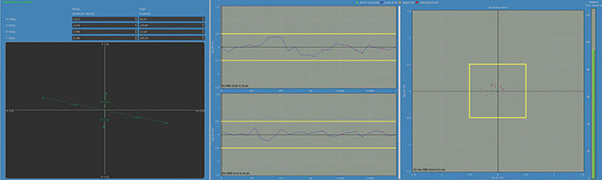
The right-hand pane of Figure 8 shows the actual guiding errors. TSIE can show whether the guide star is starting to saturate using red markers, and there are a few shown here as I used the same calibration star for autoguiding. The graphs here look jagged, suggesting poor guiding, but in fact a lot of this jitter is probably from atmospheric seeing. I’m using an off-axis guider and it’s sampling the sky through a 1,340mm focal length telescope, so it’ll certainly see some jitter. The vertical scale of this graph is in increments of 0.5 pixels and I’ve marked the first ± 0.5 pixel line in yellow. You can see from this that the guiding corrections are very small and should produce great star images in long exposures. Next, I calibrated the mount using ‘pulse’ guiding (with my Paramount ME it’s known as ‘Direct Guide’). As mentioned previously, this dispenses with a relay cable, and corrections are controlled exclusively by the mount itself. Rather than choosing a calibration value in seconds, Direct Guide requires a measurement in arcseconds. The same scenario applies as earlier, in that there must be enough movement visible without driving the star off the sensor. I found that 120 arcseconds worked well, with the calibration vectors shown in green on the left-hand of Figure 9. The centre pane shows the guiding errors with the 0.5 pixel marker line highlighted in yellow. The right-hand pane shows an RA versus Dec scatter plot with my yellow box showing vertical and horizontal guiding errors contained within the 0.5 pixel box. Happy days!
This concludes the rather intense second night, but TSIE came through with flying colours. Next issue I will use everything I’ve learned so far to take some images and look into some more new features.
At a glance
Minimum system requirements
macOS: 2GHz Intel Core Duo or faster, macOS Sierra (10.12), High Sierra (10.13), Mojave (10.14) or Catalina (10.15) 512MB RAM, 64MB video RAM, 2.5GB disk space
Windows: 1.5GHz or faster, Intel Pentium 4, Pentium M, Pentium D or better, or AMD K-8 (Athlon) or better, Windows 10, 512MB RAM, 128MB video RAM, 2.5GB disk space
Linux: A computer running 64-bit x86 Linux Ubuntu 12.04 LTS or later, Ubuntu GUI and OpenGL, 512MB RAM, 2GB minimum disc space
Raspberry Pi: Third-generation Raspberry Pi device (Raspberry Pi 3 Model B or later) SanDisk Ultra PLUS 16GB microSDHC UHS-1 card, 2GB minimum free space, Well-ventilated project case (fan not necessary) Optional external 9-pin serial port
Price: $595
Details: bisque.com