Back in the July 2018 issue of Astronomy Now, I reviewed The Sky X Professional software with an emphasis on deep-sky imaging. The Sky planetarium package has been available for many years, and each edition has incorporated many new and exciting features. For example, more recent versions introduced the ability to control imaging devices via a ‘Camera Add-on’, which could be purchased separately. Another addition was TPoint, which is equatorial-mount-modelling software, legendary for its capability to improve telescope pointing and used on several professional telescopes.
My 2018 review focused on the capabilities and ease-of-use of the Camera Add-on, since I’d already used TPoint, my being a long-time fan of The Sky X. After a few nights in my back-garden observatory, I was extremely impressed with the performance and capabilities of the package. It certainly seems to make sense to control everything from within the same software. A recent advertisement in Astronomy Now alerted me to a new release of the package, now named The Sky Imaging Edition (TSIE), and Software Bisque, the US company that supplies the software, kindly allowed me to download the full imaging package for this review. It seems that the reasoning behind this new release is that the Camera Add-on and TPoint are now included in the price, and the new version works out slightly cheaper. At the time of writing the software costs approximately £465 ($100 for the first year’s subscription, plus a $495 one-time sign-up fee). While this isn’t insignificant, it is actually very good value for money since this is a very comprehensive imaging and planetarium package.
Installation was seamless and allowed the retention of user-definable features from earlier versions, such as field-of-view indicators, as well as the panoramic view of my back garden that I’d used previously to personalise my observing location. The planetarium display looks great, is easy to use and is very customisable. Overall, the program is pretty much the same to look at as the earlier version, but I did spot some new features, which I’ll come to later. Since the earlier review, I’d carried out an upgrade from Windows 7 to Windows 10 and, during that procedure The Sky X had lost the ability to see my imaging camera. This wasn’t a showstopper as I was able to use the software’s own ASCOM driver to control the camera. Happily, after the upgrade the camera was accessible again using the native QSI drivers.
Set-up
During a welcome run of three consecutive clear and steady nights in mid-September I was able to try out the new package for deep-sky CCD imaging. I’d recently purchased a ‘previously enjoyed’ QSI 683wsg CCD camera, and it was this that I used for the review, rather than my old stalwart QSI 583wsg camera. During the daytime I was able to quickly configure the other observatory equipment. My imaging mount for the past ten years has been a Paramount ME along with a GSO 254mm (10-inch) Ritchey–Chrétien telescope fitted with an Astro-Physics 0.7× focal reducer, giving a focal length of 1,440mm. The QSI 683 camera has an internal eight-position filter-wheel, loaded with LRGB and narrowband filters, which is controlled via the camera driver. I also used a trusty Starlight Xpress Lodestar auto-guiding camera attached to the QSI 683’s integral off-axis guider port. The sensitivity of the guide camera allows the acquisition of a suitable guide star on every occasion. I’m also using a Moonlite two-inch electronic focuser that is operated via a Lakeside controller. This was set up using the ASCOM protocol in The Sky Imaging Edition software. Happily, everything connected flawlessly, which was a great relief.
First night
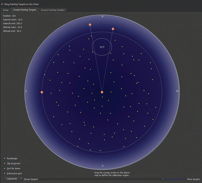
My plan was to spend the first night creating a new pointing model for the telescope. Although I have used TPoint for many years, I have never been able to get a really good model that I was satisfied with. Of course, if anything is physically changed in the imaging system, even by a small amount, then the model is degraded. The installation of the new camera and rebalancing of the mount would have done this, so it was definitely time for a new model. The methodology behind TPoint is very complex but the user-interface is relatively straightforward. There are two ways of building a pointing model. The manual method requires that the telescope be pointed to a star and an image taken. The star will most likely be offset from the sensor’s centre position by some small amount, depending on the quality of the equatorial mount used. The star can be centred using the mount’s hand-controller or via software centring (I always have a set of crosshairs on the screen to help align the star). When centred, the ‘Add Pointing Sample’ button is pressed. This is repeated many times with the telescope pointing at a large selection of stars, spread evenly across the sky and either side of the meridian to build up a record of all the potential mechanical and mount-pointing errors in the system. Alternatively, and much better, is to use the ‘Automated Pointing Calibration Run’ approach. A certain amount of information has to be provided, such as exposure time (I used three seconds), the image scale in arcseconds per pixel, binning, and so on. Next, you choose how many stars to use for the automated run, using the menu shown in Figure 1. The slider at the bottom of the screen is dragged to the left for fewer stars to be used in the model, and to the right for more stars. The area of sky used for modelling stars can be adjusted using the orange button shown at centre-left, which expands or contracts the blue circle, allowing stars close to the horizon to be excluded. After doing all this I ended up with a pointing run of 62 stars, which is probably the lower end of an ideal model, but it was a good starting point. There are four tick boxes shown at the lower left. ‘Randomize’ creates, unsurprisingly, a random but well-spaced set of stars and is recommended in the user manual. I clicked on ‘Sort for Dome’ as I assumed this would create a logical path for the stars across the sky, making movement of the dome aperture less frequent, but this didn’t seem to be the case. I’d planned to incorporate a five-second delay between star images to allow more time to move the dome, but in my excitement I forgot, so I ended up scrambling around trying to keep up with the slewing telescope.
Plate-solving problems
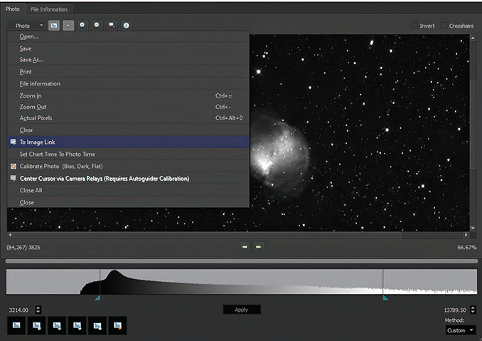
Proceeding to the next tab, ‘Acquire Pointing Samples’ displays a vertical list of the chosen stars. Clicking on the ‘Run’ button starts the procedure. The telescope slewed to the first star, took an image, attempted to ‘plate-solve’ but then failed. Plate-solving is where the stars in an image are plotted and then matched with a large database of stars from a catalogue. Once successful, the mount’s position is known with great accuracy. Unfortunately, after the first failure the mount slewed to the next star and also failed. This was a source of confusion since the ‘FITS Viewer’ window (more on this window later) allows the stars in the image to be plate-solved by the observer using the ‘To Image Link’ option from the drop-list, shown in Figure 2. Image Link is what The Sky calls plate-solving. When I tried this, it worked perfectly. I revisited the earlier setup menus and after a bit of head-scratching unticked the ‘Use All Sky Image Link for automated pointing runs’ box and thankfully everything worked fine after that. I subsequently discovered that there is an ‘All Sky Database’ file available for download from the Software Bisque website that can be installed in the ‘Astrometry’ folder of TSIE and which may fix the issue. Over the next 45 minutes or so the mount continued to slew around the sky and acquired 61 pointing samples. The lone failure was because of my not being fast enough with the dome. The frenetic path of the telescope around the sky is shown in Figure 3, with the filled yellow dots marking the positions of the stars used for the modelling run.

When the pointing run is completed the results are amalgamated into a ‘supermodel’ that improves the pointing further. Figure 4 shows the results after the supermodel was applied. The inner circle of the scatter plot at top left measures 36.3 arcseconds and contains the majority of the 61 pointing samples. TPoint can also give a precise polar-alignment assessment based on the model. Clicking on the ‘Polar Alignment’ tab shows the result. It seems that my azimuthal adjustment is slightly out but the altitude adjustment is very good. TPoint states how much the mount has to be adjusted and in which direction, but another model would be required, so I left it alone (Figure 5).

Amazing accuracy
By this point I was quite keen to see how well the telescope was pointing, so I slewed it onto M27, the Dumbbell Nebula in Vulpecula. The left-hand pane of Figure 6 shows the placement of M27 after the first slew. This is a highly magnified view of the central area of the CCD sensor and you can see the central star of the planetary nebula just to the lower left of the crosshair’s centre point. This certainly represents great pointing accuracy and I’d feel no need to position this any better before starting an imaging run. The full sensor is shown in the small image at lower-middle.
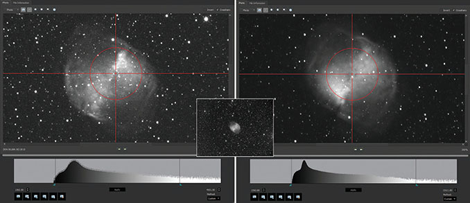
I revisited M27 later, after it had crossed the meridian, so that the mount had to carry out a full meridian flip, rotating through 360 degrees to approach the target from the opposite side of the sky. When the image downloaded I was amazed at the positional accuracy. The central star is shown just fractionally below the crosshair’s centre point in this flipped image (right-hand pane of Figure 6).
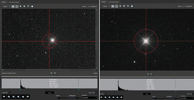
There are a couple of points worth mentioning here. Figure 7 shows the bright star Caph (beta Cassiopeia) that I’d used as a pointing test after the TPoint run. It’s displayed in TSIE’s ‘FITS Viewer’ screen. Once an image has been taken and downloaded, it is automatically opened in this viewer. A red crosshair can be turned on using the tick-box at the top right. After the initial slew, the star was placed almost on the crosshair, again representing great pointing accuracy. This can be refined even more by using a feature called ‘Closed Loop Slew’, which isn’t new to the latest edition but is definitely worth using. Here’s how it works. A star or deep-sky object is chosen using the ‘Find’ tab on the left of the main screen. Once found, a lot of information is displayed, including right ascension, declination, rise time, transit time, and so on. Next, click on ‘Closed Loop Slew’ and the mount will slew to the target, take an image and then Image Link it (plate-solve). Once done, the mount is shifted to centre the target and then another image is taken. When the image is downloaded, the target should be smack bang on the centre of the image (see right-hand pane of Figure 7). You can also choose how the image is displayed. The ‘Show Histogram’ button at top-left, next to the ‘Photo’ tab, opens the image-scaling options across the bottom of the menu and at bottom-right is a drop-list containing several options. The first is ‘SBIG’, and anyone who has owned a Santa Barbara Instruments Group CCD camera will be familiar with its display properties. Two sliders, labelled ‘Scale’ and ‘Highlights’, and a histogram are shown and these can be manipulated to give good shadows and brightness values, particularly important if you are manually focusing on a star. A new option in the list caught my eye, intriguingly named ‘Heuristic’. Clicking on this changes the display quite dramatically and gives a view that resembles one obtained with Digital Development Processing, logarithmic scaling or the ‘auto stretch’ feature in PixInsight. I also used it when checking the autofocus capabilities (more of which in the next issue) because it showed stellar diffraction spikes very clearly. Figure 8 shows a monochrome 10-minute exposure of M27 using the SBIG option on the left and Heuristic on the right.

It was a fantastic first night. In the next issue we’ll chronicle how the software performed during the second night, and in particular assess the autofocus and auto-guiding capabilities of The Sky Imaging Edition.
At a glance
Minimum system requirements
macOS: 2GHz Intel Core Duo or faster, macOS Sierra (10.12), High Sierra (10.13), Mojave (10.14) or Catalina (10.15) 512MB RAM, 64MB video RAM, 2.5GB disk space
Windows: 1.5GHz or faster, Intel Pentium 4, Pentium M, Pentium D or better, or AMD K-8 (Athlon) or better, Windows 10, 512MB RAM, 128MB video RAM, 2.5GB disk space
Linux: A computer running 64-bit x86 Linux Ubuntu 12.04 LTS or later, Ubuntu GUI and OpenGL, 512MB RAM, 2GB minimum disc space
Raspberry Pi: Third-generation Raspberry Pi device (Raspberry Pi 3 Model B or later) SanDisk Ultra PLUS 16GB microSDHC UHS-1 card, 2GB minimum free space, Well-ventilated project case (fan not necessary) Optional external 9-pin serial port
Price: $595
Details: bisque.com